OptimEFE v2.2

The application field of OptimEFE is to solve the two main technical problems which are related to function minimizing and least square optimization (curve fitting of arbitrary dimension).

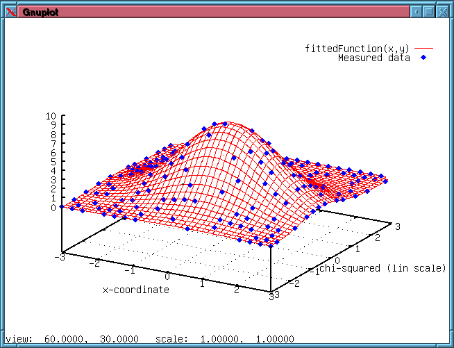
The least square optimization is available since version 2.0.

OptimEFE was written to close the gap between a pure numerical packages like 'matlab, octave,..' on the one side and external simulators on the other side. These external simulators response to a request which is defined by the binary OptimEFE. To exchange the data the external simulators have to write the calculated results in a readable text file.

On the one hand OptimEFE consists of a single C-file (OptimEFE.c) which represents after compilation the numerical optimizer. On the other hand this compiled binary can extract example files which set up a complete optimization environment.  

Example of a schematic flow of the OptimEFE optimization environment. The shell script controls the flow and call the needed binaries. For more infos check out the OptimEFE user manual.

The job of the binary OptimEFE is to define the independent points for gradient calculation and line minimization, and the external simulator corresponds to the function evaluation. In reality the function evaluation is often very time consuming (e.g.finite element (FEM) simulators,..) and therefore one optimizer cycle is defined by a gradient calculation or by a line minimization. OptimEFE is written to do all necessary calculations of one cycle in parallel. In case a problem has five independent variables, all five external simulator calls for the gradient calculation are done in parallel and in the next cycle (which is a line minimization) all specified line points are calculated in parallel.

OptimEFE provides an interactive mode where the file 'optimizerControl' can be modified for each iteration before it is read. This allows to change values like parameter boundaries and to control the optimization process in an interactive way. This is especially useful for time consuming external evaluation which helps to minimize the overall optimization time.

To use the full functionality of the optimization environment the tools 'bash' 'gnuplot' and 'gawk' are needed.

OptimEFE was alo tested under the Cygwin environment. In this environment it is possible to call MS-Windows programs and use the OptimEFE file flexibility for the data exchange. Again the windows program (e.g. FEM software) which calculates the response must write a result file in a text format.

The scope of OptimEFE is to define next experiments and to start new job requests. Normally the new job requests are sent to a load balancer which again send the jobs to different machines. OptimEFE does not control the load and also license and server farm issues are not scope of OptimEFE.

OptimEFE version 2.0 was tested using the linux distributions listed below:

For further information check out the OptimEFE user manual.

Keywords: optimization, external function binding, external function evaluation, global optimization, FEM, TCAD

Function minimizing:

To solve ill-conditioned problems OptimEFE is based on the conjugate gradient approach. Also a simple steepest gradient optimization can be specified. For all independent variables valid ranges must be specified. Often the independent variables cover different orders of magnitudes (e.g. ion implant dose (1e15cm-2), distances (1e-6m). Therefore OptimEFE normalize all independent variables for the internal calculation. Also a logarithmic scaling of the independent variables can be specified. This is useful for variables with a positive variable range (e.g. temperature, time, concentration,...). After specifying the new cycle points OptimEFE stores the information in the file 'optimizerOutput' and exit. The results from the function evaluation are stored in the file 'optimizerInput'. Together with the file 'optimizerControl' OptimEFE is called again. Using these two files OptimEFE gets into the old state and goes on the optimization.

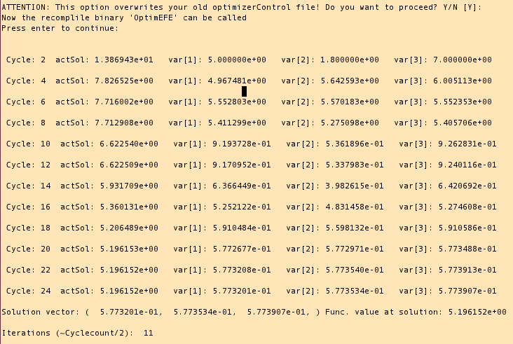
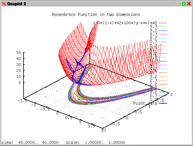
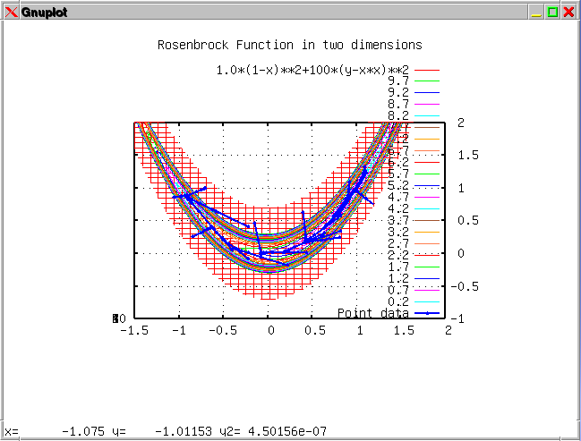
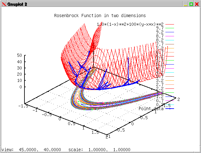
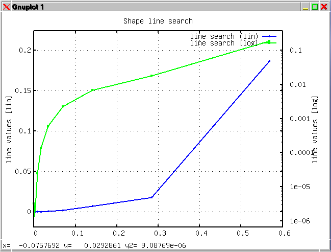
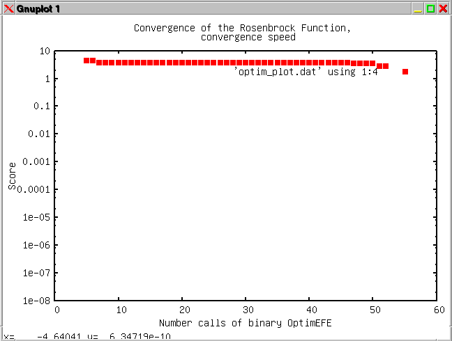
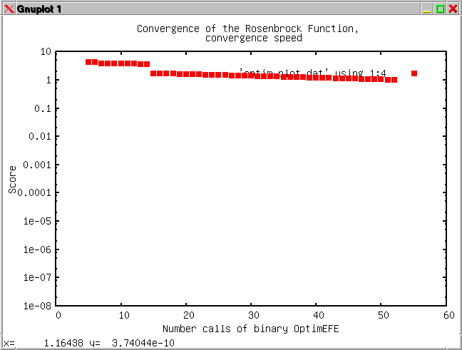
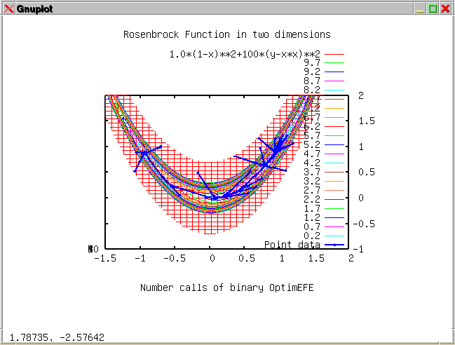
After compiling OptimEFE one can extract six examples (shell scripts) for function minimizing (command: 'OptimEFE -generateExampleFiles').

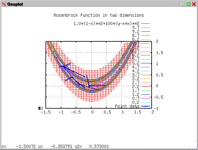
• The first examples uses an internal function evaluation. Therefore the source file OptimEFE.c is modified to define the new function, is recompiled and executed.

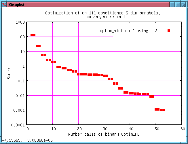
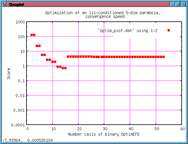
• The second example evaluates an external function with GNU awk. The results can be extracted from the file 'optimizerLog'. The examples optimizes an ill-conditioned parabola with 5 independent variables.

• The third example again uses an external function. In contrast to example2 the external simulator binding is much more sophisticated. For each function evaluation a new directory is created which name holds the independent variable values. In these directories a number of result values are calculated but the final function value is calculated again in the optim_example3 batch file.

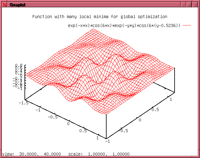
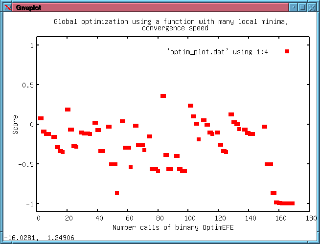
• The fourth example shows a global optimization of a function which has several local minima. The global search is done by splitting the complete function range in small areas and do a minimization on every sub-area. Finally the sub area with the lowest function value is used for a final minimization with a higher accuracy.

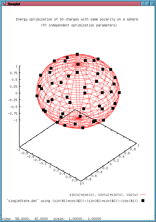
• The fifth example shows a multidimensional optimization of charges on a sphere. The result is a charge distribution in a minimum electrostatic energy state. The example demonstrates that problems up to 100 optimization parameters can be handled with OptimEFE.

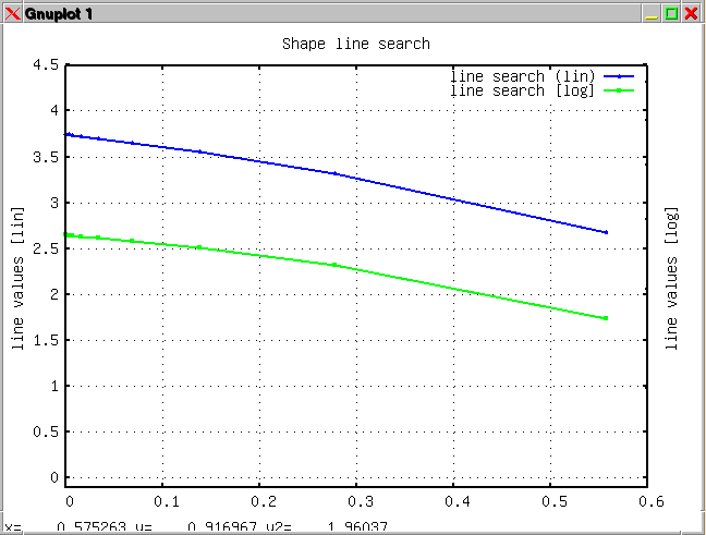
• The sixth example is similar to example number one except that the evaluation is done with an external function. The example compares the conjugate gradient with the steepest gradient approach combined with a logarithmic or linear scaling of the independent variables (side lengths).

  
  

Examples for function minimizing:

Least Square (LS) Optimization:

In case of one independent variable this optimization task is labeled as curve fitting. It is important to know that the LS optimization is independent of the number of the independent variables. In case of OptimEFE the optimizer has no information about the number of independent variables because the function is evaluated externally. Only the number of optimization parameters are available and OptimEFE defines the new parameter sets by calculating the parameter gradients. In case of N optimization parameters and M sample data points, OptimEFE requests about (N+1)*M function values before OptimEFE terminates and the external function evaluation is started.

The implemented LS algorithm uses the Levenberg-Marquardt approach for the optimization. The algorithm allows to specify a damping using the damping factor 'lambda'. To guarantee a correct result the damping parameter has to become zero when the parameters are close to the final solution. This is achieved by a two step approach where two successive steps are compared. In case the sum of the new least square values (chisq) are smaller than the old chisq value, lambda is reduced by a certain factor. In case the new chisq is larger tan the old chisq lambda is increased.

After compiling OptimEFE one can extract three examples (shell scripts) for least square  minimizing (command: 'OptimEFE -generateExampleFiles').

• The first example shows a two joined half Gaussian function which is frequently used for e.g. ion implant profiles. The examples shows a piecewise defined function with 8 optimization parameters.

• The second example demonstrates the optimization of a function with two independent variables and 5 optimization parameters. It also demonstrates the graphical flexibility of gnuplot.

• The third example describes is a more general curve fitting problem where a number of joined parabolas of degree 3 can be specified. The example demonstrates that problems up to 100 optimization parameters can be handled with OptimEFE.

Examples for least square minimizing: